
The following video highlights the key steps to exporting student activity reports and coverting them into spreadsheets to analyze the data in tables.
Click the Play button below to get started.
Exporting Pulse Student Activity Report
Navigate to the Reports tab in Pulse and select Student Activity Report.

Filter the report as needed.
TIP: If you have more than one school associated to your district, click on the School Name filter, select the desired school, and click OK.

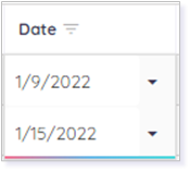
In the Date column, click on the magnifying glass and select Between.

TIP: After selecting Between, click in the search field to populate Start and End date options.
Select the Start and End dates.
Click on Export to pull the results into an Excel file.

This Excel file will allow you to create PivotTables in both Excel and Google Sheets.
Adjusting Excel Data to a PivotTable
Open the Excel file exported from Pulse.
NOTE: If prompted, click on Enable Editing.
TIP: If needed, select all the rows in the Minutes column and convert to a Number value.

Select all the data within the report.

IMPORTANT: Do not select blank columns or rows.
In the top ribbon of Excel, click Insert, then PivotTable.

Click OK in the Create PivotTable window.

In the PivotTable Fields, choose the data you want to reflect.
The below example uses the PivotTable Fields in the Field Section and Areas Section Stacked view.

To see total time per student, select Student Full Name and Minutes.

To see subtotals of time per student per course, select Student Full Name, Class Name, and Minutes.

TIP: Select Last Activity Name if you want to list the last activity the student visited by Class Name.

Beneath the Choose fields section, you will see where you can drag fields for Filters, Columns, Rows, and Values.
IMPORTANT: Make sure Minutes is found in Values and the action is set to Sum.

You can adjust these details by clicking the drop-down arrow and selecting a specific action. You can also drag and drop as needed.

Select Value Field Settings if you need to adjust the value action.

PivotTable Outcomes
Once you apply a PivotTable, you will see the outcomes in the newly created Sheets tab. Below are examples of the two different setting outcomes.
Student Full Name and Minutes

Student Full Name, Class Name, and Minutes

Using the Excel Data to Create a Pivot Table in Google Sheets
In your Google Drive, select +New.

From the pop-up menu, select File upload.

Choose the Excel file and click Open to upload this file to your Google Drive as a Google Sheet.

Open your newly uploaded Google Sheet and highlight all the rows in the Minutes column.

Click Format, and from the Number pop-up menu, click Number.

Select all the data within the report.

IMPORTANT: Do not select blank columns or rows.
Click Insert, and then select Pivot table.

Click Create to have your pivot table created in a new sheet within your report.

In the Pivot table editor, choose the data you want reflected.
To see total time per student, beside Rows, click Add and select Student Full Name.

Next, beside Values, click Add and select Minutes.

IMPORTANT: Make sure to Summarize by Sum.

To see subtotals of time per student per course, drag Class Name from the Search column and drop underneath Student Full Name in Rows.

TIP: Drag and drop Last Activity Name under Class Name to see the last activity the student visited by class name.
Pivot Table Outcomes
Once you begin using the Pivot table editor, you will see the outcomes in the newly created Sheets tab. Below are examples of the two different setting outcomes.
Student Full Name and Minutes

Student Full Name, Class Name, and Minutes

Please note the images found in this resource may not match your screen. Access and/or features may vary based on client contract.
© 2025 Lincoln Learning Solutions. All rights reserved.